The recent warming has been more pronounced in the Arctic Eurasia than in many other regions on our planet, but Franzke (2012) argues that only one out of 109 temperature records from this region exhibits a significant warming trend. I think that his conclusions were based on misguided analyses.
The analysis did not sufficiently distinguish between signal and noise, and mistaking noise for signal will give misguided conclusions.
We must know how random year-to-year variations compare to the long-term warming in order to determine whether a trend is statistically significant. The year-to-year variations are often referred to as noise, whereas the trend is the signal.
Franzke examined several models for describing the noise. These are referred to as null models. One involved the well-known lag-one autocorrelation (AR(1)). Another null model was an ARFIMA model, similar to Cohn and Lines. The third null model involved phase scrambling surrogate model (see below for details).
He examined the autocorrelation functions (ACF) of fitted noise models with the autocorrelation of the temperature records, and found that the ACF for phase scrambling was the same as for the original data. This similarity is expected, however, due to the fact that the phase scrambling preserves the spectral power.
The fact that the ACFs were similar for the data and the null model is also a clue for why the analysis is wrong. The ACF for the temperature data included both signal and noise, whereas the null models are only supposed to describe the noise. Moreover, the null models in this case derived the long-term persistence from a combination of the signal and noise.
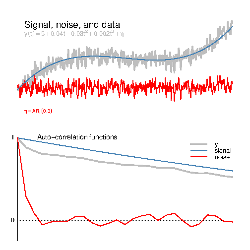
The mixing-up between signal and noise is illustrated in the example below, where the variable y was constructed from a signal component and a noise component. The lagged correlation coefficients of the grey ACF estimated from y were substantially higher than those for the AR(1) noise (red), due to the fact that the signal contained a high degree of persistence.

ACF for a series 'y' (grey) constructed from a 3rd-order polynomial (blue) and AR(1) noise (red). In this example, the polynomial is the signal and the AR(1) is the noise. Note that the ACF for the sum of these two components is different to the ACF for the noise term. The y-axis of the lower panel represents correlations whereas the x-axis marks the time lag.The phase scrambling will give invalid estimates for the confidence interval if the low frequencies represent both the signal and noise. Even the ARFIMA model is invalidated by the presence of a signal if it is used to describe confidence intervals. The problem is similar to the weakness in the analysis of Cohn and Lins discussed in the ‘Naturally Trendy?‘ post. Hence, both these null models over-estimate the amplitude of the noise. Alternatively, it may be a question about definition: if one defines the trend itself as noise, then it will not be statistically significant (circular reasoning).
Details
The third null model involved a Fourier transform, followed by changing the Fourier coefficients while ensuring that the spectral power stays the same, and then by an inverse Transform.
The analysis did not sufficiently distinguish between signal and noise, and mistaking noise for signal will give misguided conclusions.
We must know how random year-to-year variations compare to the long-term warming in order to determine whether a trend is statistically significant. The year-to-year variations are often referred to as noise, whereas the trend is the signal.
Franzke examined several models for describing the noise. These are referred to as null models. One involved the well-known lag-one autocorrelation (AR(1)). Another null model was an ARFIMA model, similar to Cohn and Lines. The third null model involved phase scrambling surrogate model (see below for details).
He examined the autocorrelation functions (ACF) of fitted noise models with the autocorrelation of the temperature records, and found that the ACF for phase scrambling was the same as for the original data. This similarity is expected, however, due to the fact that the phase scrambling preserves the spectral power.
The fact that the ACFs were similar for the data and the null model is also a clue for why the analysis is wrong. The ACF for the temperature data included both signal and noise, whereas the null models are only supposed to describe the noise. Moreover, the null models in this case derived the long-term persistence from a combination of the signal and noise.
The mixing-up between signal and noise is illustrated in the example below, where the variable y was constructed from a signal component and a noise component. The lagged correlation coefficients of the grey ACF estimated from y were substantially higher than those for the AR(1) noise (red), due to the fact that the signal contained a high degree of persistence.

ACF for a series 'y' (grey) constructed from a 3rd-order polynomial (blue) and AR(1) noise (red). In this example, the polynomial is the signal and the AR(1) is the noise. Note that the ACF for the sum of these two components is different to the ACF for the noise term. The y-axis of the lower panel represents correlations whereas the x-axis marks the time lag.
Details
The third null model involved a Fourier transform, followed by changing the Fourier coefficients while ensuring that the spectral power stays the same, and then by an inverse Transform.
References
C. Franzke, "On the statistical significance of surface air temperature trends in the Eurasian Arctic region", Geophysical Research Letters, vol. 39, 2012. http://dx.doi.org/10.1029/2012GL054244
DIGITAL JUICE
No comments:
Post a Comment
Thank's!